Training#

mbGDML is a data-driven method, meaning we need to train an ML model to reproduce a system’s potential energy surface (PES). Once we have a collection of structures (usually from an MD simulation) and calculated energies and forces, we can begin training GDML models.

Data#

We require data to be stored in NumPy npz files. These are binary files that can store several NumPy arrays of various types. At a minimum, mbGDML needs four arrays containing information about the PES.

Z of shape (n_atoms,): atomic numbers for all structures in the data set.
R of shape (n_structures, n_atoms, 3): Cartesian coordinates of all structures in the data set.
E of shape (n_structures,): Total or many-body energy for each structure.
F of shape (n_structures, n_atoms, 3): Total or many-body atomic forces for each structure.

Attention

GDML uses a global descriptor, meaning the number and order of atoms must be the same for each structure. For example, if you have a single water molecule and your Z is [8, 1, 1], then every structure in R must have the oxygen atom first.

Here are some examples of water 1-body, 2-body, and 3-body data sets.

Tip

Sampling, curating, and calculating data sets is done with a complementary Python package reptar. Please refer to reptar’s documentation.

Data set class#

We use the DataSet class to load and provide simple access to data.

Note

We will frequently use Z, R, E, and F as the key in the npz file for their respect data. You can load data sets by passing X_key when initializing the DataSet class. For example, you can have Z_key be 'atomic_numbers'.

What are we training?#

The underlying technical details of GDML are essential, but only a few concepts are necessary for training and using models. Briefly, a GDML model takes Cartesian coordinates and outputs energy and forces shown in the following flowchart.

flowchart LR coords[/Coordinates/] --> desc[/Descriptor/] desc -- sigma --> traindist[/Train set</br>distances/] traindist -- alphas --> forces[/Forces/] forces -- integ_c --> energy[/Energy/]

sigma, alphas, and the integration constant integ_c are the three data pieces we get during training for predictions. We will discuss these later.

Matérn kernel#

GDML is based on the Matérn kernel, \(k_\nu\), that is twice differentiable (\(\nu = 5/2\)):

(1)#\[k_{5/2} (\overrightarrow{x}_i, \overrightarrow{x}_j) = \left( 1 + \frac{\sqrt{5}}{\sigma} d(\overrightarrow{x}_i, \overrightarrow{x}_j) + \frac{5}{3\sigma} d(\overrightarrow{x}_i, \overrightarrow{x}_j)^2 \right) \exp \left( - \frac{\sqrt{5}}{\sigma} d (\overrightarrow{x}_i, \overrightarrow{x}_j) \right),\]

where \(\overrightarrow{x}_i\) and \(\overrightarrow{x}_j\) are the descriptors of two data points \(i\) and \(j\), \(\sigma\) is the kernel length scale, and \(d (\overrightarrow{x}_i, \overrightarrow{x}_j)\) is the L2 (i.e., Euclidean) norm or distance between \(\overrightarrow{x}_i\) and \(\overrightarrow{x}_j\).

Note

GDML literature uses \(\sigma\) to represent kernel length scale. \(l\) is often used in other sources.

GDML uses the inverse atomic pairwise distances as the descriptor (e.g., \(x_i\) and \(x_j\)). For example, consider this water dimer.

We can compute the inverse atomic pairwise distances with _from_r() (and their partial derivatives needed for GDML models).

import numpy as np
from mbgdml._gdml.desc import _from_r

# Water dimer coordinates.
R = np.array(
    [[ 1.80957202,  0.78622087,  0.4170556 ],
     [ 1.39159092,  0.9217478 ,  1.27126597],
     [ 2.40137633,  0.04199757,  0.55361951],
     [-0.16942685,  0.19603795, -1.64383542],
     [-0.10053189,  0.84679289, -2.34463743],
     [ 0.50972947,  0.45598791, -1.00676722]]
)
# Compute the pairwise descriptors and their partial derivatives.
r_desc, r_desc_d = _from_r(R)
print(r_desc)  # Descriptor
# [1.04101674 1.04101716 0.65814497 0.34275482 0.29538202 0.29537792
#  0.29775736 0.25559815 0.25559542 1.04293945 0.51124879 0.40212734
#  0.40211189 1.03435064 0.65723451]
print(r_desc_d)  # Descriptor partial derivatives
# [[-0.47155221  0.15289692  0.96369139]
#  [ 0.66765451 -0.83960869  0.15406699]
#  [ 0.28786826 -0.25079801 -0.20458568]
#  [-0.07968861 -0.02376498 -0.08298618]
#  [-0.04023092 -0.01870317 -0.07512869]
#  [-0.0662526   0.0039698  -0.05663098]
#  [-0.05042484  0.00159904 -0.07290594]
#  [-0.02491596 -0.00125162 -0.06037956]
#  [-0.04177636  0.01343831 -0.04839451]
#  [ 0.07815643  0.73823522 -0.79501006]
#  [-0.17369512 -0.04412831 -0.19026234]
#  [-0.05734442 -0.03028677 -0.14813267]
#  [-0.12299311  0.02691727 -0.10145489]
#  [ 0.75157635  0.28766903  0.70500027]
#  [ 0.17325148 -0.11094843  0.37981758]]

Note

Predictions using GDML do not directly use _from_r() but instead uses Desc.

Important

GDML does not directly use or compute the Matérn kernel. Instead, it uses the Hessian matrix of the Matérn kernel where each row and column encodes how a training point “interacts” with all other training points. We will refer to this as the kernel matrix. _assemble_kernel_mat() and _assemble_kernel_mat_wkr() are used to build this.

`sigma`#

The kernel length scale, \(\sigma\) or sigma, is the hyperparameter we optimize during training from Equation (1). It broadly represents the smoothness of how quickly the kernel function can change. As we can see in the figures below, the smaller length scale rapidly changes to better fit the data.

http://evelinag.com/Ariadne/img/smallLengthscale.png — Small length scale.#

http://evelinag.com/Ariadne/img/largeLengthscale.png — Large length scale.#

There is no analytical way to determine the optimal sigma. We have to iteratively try values that minimizes the error during training. How we do this in mbGDML will be discussed later.

`alphas`#

Once we have the kernel Hessian, we need the (n_train, n_atoms, 3) regression parameters. This is analytically determined using Cholesky factorization. First, we use scipy.linalg.cho_factor() to decompose the negative kernel matrix from _assemble_kernel_mat() after we apply the regularization parameter lam: K[np.diag_indices_from(K)] -= lam. The negative of scipy.linalg.cho_solve() computes alphas where the targets are the atomic forces (scaled by their standard deviation). If Cholesky factorization fails, we try LU factorization with scipy.linalg.solve().

(2)#\[\hat{\boldsymbol{f}}_\boldsymbol{F} (\overrightarrow{x}_i) = \sum_i^M \sum_j^{3N} \left( \overrightarrow{\alpha}_i \right)_j \frac{\partial}{\partial x_j} \nabla_{\overrightarrow{x}_i} \: k_{5/2} (\overrightarrow{x}_i, \overrightarrow{x}_j)\]

All of this is automatically done in Analytic.

`integ_c`#

GDML is an energy-conserving force field where the energy is recovered by integrating the forces up to an integration constant, integ_c.

(3)#\[\hat{f}_E (\overrightarrow{x}_i) = \sum_i^M \sum_j^{3N} \left( \overrightarrow{\alpha}_i \right)_j \frac{\partial}{\partial x_j} k_{5/2} (\overrightarrow{x}_i, \overrightarrow{x}_j) + c\]

This is automatically done in _recov_int_const().

Training routines#

We provide a class, mbGDMLTrain, that manages all training routines. All you need to do is initialize mbGDMLTrain with the desired options and then pick one of the following routines to train a model:

The primary difference between these two routines is how an optimal sigma is selected. grid_search() is a brute-force routine where it selects the model with the lowest validation loss from each sigma in sigma_grid. bayes_opt() takes this a step further and uses Bayesian optimization of sigma around the region identified by a preliminary grid search.

`create_task`#

create_task()

flowchart LR mbGDMLTrain([mbGDMLTrain]) -- sigma --> create_task([create_task]) create_task --> task[/Task/]

`train_model`#

train_model()

flowchart LR task[/Task/] --> train_model([train_model]) train_model --> model[/Model/]

`add_valid_errors`#

flowchart LR model[/Model/] --> add_valid_errors([add_valid_errors]) add_valid_errors --> errors[/Validation<br/>errors/]

`sigma` optimization#

mbGDML provides two standard routines for optimizing sigma: grid_search() and bayes_opt()

`grid_search`#

grid_search() performs a simple grid search on the sigmas provided in sigma_grid. Typically, the validation errors will decrease with increasing sigmas and eventually start rising. So we sort the sigmas by ascending values and repeat the training routine discussed above until the validation errors begin to rise.

_images/1h2o-sigma-loss-increasing.png — Validation loss, `loss_f_e_weighted_mse()`, of training a water 1-body force field with 1000 training points. Note: additional `sigmas` were performed for illustrative purposes.#

Info

This is how the sGDML package trains their models.

`bayes_opt`#

More often than not, the optimal sigma is not one in sigma_grid, but somewhere in between. We implemented a routine using the bayesian-optimization, package that better optimizes sigmas. Furthermore, unlike the sGDML package we do not restrict sigma to integer values.

_images/2h2o-sigma-dual-min.png — Validation loss, `loss_f_e_weighted_mse()`, of training a water 2-body force field with 300 training points.#

Active learning#

active_train()

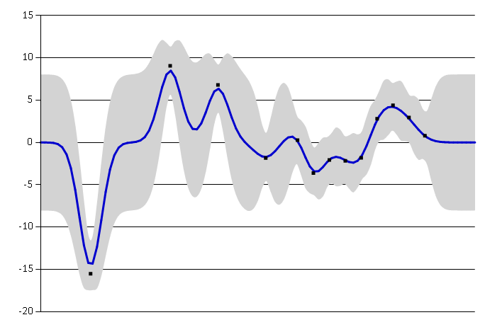
_images/1h2o-cl-losses-1000-rand.png — Mean loss, `loss_f_mse()`, from a randomly trained water 1-body model on 1000 structures. An initial model was trained on `100` structures and `50` structures were iteratively added until `1000` was reached. The maximum cluster loss was \(0.163\) [kcal/(mol A)]².#

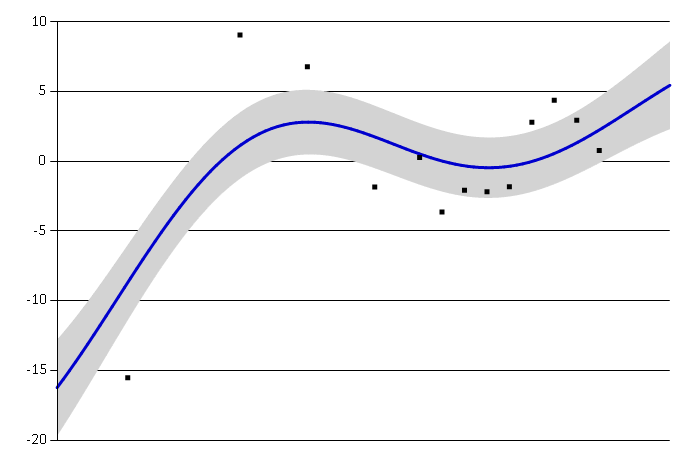
_images/1h2o-cl-losses-1000-iter.png — Mean loss, `loss_f_mse()`, from a water 1-body model trained with active learning on 1000 structures. Structures were automatically selected using `draw_strat_sample()`. The maximum cluster loss was \(5.079 \times 10^{-7}\) [kcal/(mol A)]².#

Examples#

Water 3-body#

These examples demonstrate different procedures to train a 3-body water model using the mbGDMLTrain interface. All examples below can be used with this dataset.

Active learning#

The script below shows an example of using active_train() for a 3-body water model. Here is an example dataset and model.

import os
from mbgdml.data import DataSet
from mbgdml.train import mbGDMLTrain
from mbgdml.losses import loss_f_e_weighted_mse
from mbgdml.utils import get_entity_ids, get_comp_ids


# Ensures we execute from script directory (for relative paths).
os.chdir(os.path.dirname(os.path.realpath(__file__)))


# Setting paths.
# dset_path: Path to dataset to train on.
# log_path: Path to directory where training will occur
#     (logs and model will be stored here).
model_name = "3h2o-nbody-model"
dset_path = "3h2o-nbody.npz"
save_dir = "./"


# System fragmentation
entity_ids = get_entity_ids(atoms_per_mol=3, num_mol=3)
comp_ids = get_comp_ids("h2o", num_mol=3)


# Loading data set
dset = DataSet(dset_path)
dset.entity_ids = entity_ids
dset.comp_ids = comp_ids


# Setting up training object
train = mbGDMLTrain(entity_ids=entity_ids, comp_ids=comp_ids, use_sym=True, use_E=True)

train.bayes_opt_params = {
    "init_points": 10,
    "n_iter": 10,
    "acq": "ucb",
    "alpha": 1e-7,
    "kappa": 0.1,
}
train.bayes_opt_params_final = {
    "init_points": 10,
    "n_iter": 20,
    "acq": "ucb",
    "alpha": 1e-7,
    "kappa": 0.1,
}
train.initial_grid = [
    2, 25, 50, 100, 200, 300, 400, 500, 700, 900, 1100, 1500, 2000, 2500, 3000,
    4000, 5000, 6000, 7000, 8000, 9000, 10000
]
train.sigma_bounds = (min(train.initial_grid), max(train.initial_grid))
train.loss_func = loss_f_e_weighted_mse
train.loss_kwargs = {"rho": 0.01, "n_atoms": dset.n_Z}
train.require_E_eval = True
train.keep_tasks = False


# Train the model
train.active_train(
    dset, model_name, n_train_init=200, n_train_final=1000, n_valid=100,
    n_train_step=50, n_test=1000, save_dir=save_dir, overwrite=True,
    write_json=True, write_idxs=True,
)

Training#

Data#

Data set class#

What are we training?#

Matérn kernel#

sigma#

alphas#

integ_c#

Training routines#

create_task#

train_model#

add_valid_errors#

sigma optimization#

grid_search#

bayes_opt#

Active learning#

Examples#

Water 3-body#

Active learning#

`sigma`#

`alphas`#

`integ_c`#

`create_task`#

`train_model`#

`add_valid_errors`#

`sigma` optimization#

`grid_search`#

`bayes_opt`#